39 add data labels to pivot chart

How to add Data label in Stacked column chart of Pivot charts Show activity on this post. I'm tring to make a Pivot chart with stacked column graph. In where, i couldn't add data label for cumulative sum of value in Data label. Where i could only add data label to individual stacks in column graph. It found possible with normal stacked column chart without pivot chart. How to Add Data to a Pivot Table in Excel | Excelchat We can Add data to a PivotTable in excel with the Change data source option. "Change data source" is located in "Options" or "Analyze" depending on our version of Excel. The steps below will walk through the process of Adding Data to a Pivot Table in Excel.. Figure 1- How to Add Data to a Pivot Table in Excel

Add the count of data to data labels to a pivot chart in excel You need to add the 'Data Labels' first for all lines. Then go to individual data labels & refer it to the cell you need by selecting one label at a time and press "=". Every time the data in the reference cells change, the data labels change too. I have updated the data labels in the attached file. Attached Images

Add data labels to pivot chart

Change the format of data labels in a chart To get there, after adding your data labels, select the data label to format, and then click Chart Elements > Data Labels > More Options. To go to the appropriate area, click one of the four icons ( Fill & Line, Effects, Size & Properties ( Layout & Properties in Outlook or Word), or Label Options) shown here. How to change/edit Pivot Chart's data source/axis/legends in Excel? Actually, it's very easy to change or edit Pivot Chart's axis and legends within the Filed List in Excel. And you can do as follows: Step 1: Select the Pivot Chart that you want to change its axis and legends, and then show Filed List pane with clicking the Filed List button on the Analyze tab.. Note: By default, the Field List pane will be opened when clicking the pivot chart. Formal ALL data labels in a pivot chart at once How do I format all data labels for all series in a chart at once? I frequently make pivot charts with multiple data series (line graphs). I know how to click on a data point and use the pane on the right to format the labels for that series, but it only changes that series.

Add data labels to pivot chart. How to add data labels from different column in an Excel chart? Right click the data series in the chart, and select Add Data Labels > Add Data Labels from the context menu to add data labels. 2. Click any data label to select all data labels, and then click the specified data label to select it only in the chart. 3. How to update or add new data to an existing Pivot Table in Excel Change the Source Data for your Pivot Table In order to change the source data for your Pivot Table, you can follow these steps: Add your new data to the existing data table. In our case, we'll simply paste the additional rows of data into the existing sales data table. Here's a shot of some of our additional data. Automatic Row And Column Pivot Table Labels Select the Insert Tab. Hit Pivot Table icon. Next select Pivot Table option. Select a table or range option. Select to put your Table on a New Worksheet or on the current one, for this tutorial select the first option. Click Ok. The Options and Design Tab will appear under the Pivot Table Tool. Select the check boxes next to the fields you want ... How to Add Data Labels in Excel - Excelchat | Excelchat After inserting a chart in Excel 2010 and earlier versions we need to do the followings to add data labels to the chart; Click inside the chart area to display the Chart Tools. Figure 2. Chart Tools. Click on Layout tab of the Chart Tools. In Labels group, click on Data Labels and select the position to add labels to the chart.

Adding rich data labels to charts in Excel 2013 - Microsoft 365 Blog To add a data label in a shape, select the data point of interest, then right-click it to pull up the context menu. Click Add Data Label, then click Add Data Callout . The result is that your data label will appear in a graphical callout. In this case, the category Thr for the particular data label is automatically added to the callout too. How to Customize Your Excel Pivot Chart and Axis Titles In Excel 2007 and Excel 2010, you use the Chart Title and Axis Titles commands on the Layout tab to add chart and axis titles. After you choose the Chart Title or Axis Title command, Excel displays a submenu of commands you use to select the title location. Add or remove data labels in a chart - support.microsoft.com To label one data point, after clicking the series, click that data point. In the upper right corner, next to the chart, click Add Chart Element > Data Labels. To change the location, click the arrow, and choose an option. If you want to show your data label inside a text bubble shape, click Data Callout. How to Customize Your Excel Pivot Chart Data Labels - dummies To add data labels, just select the command that corresponds to the location you want. To remove the labels, select the None command. If you want to specify what Excel should use for the data label, choose the More Data Labels Options command from the Data Labels menu. Excel displays the Format Data Labels pane.

Add Percentage to Pivot Table | MyExcelOnline Excel Pivot Tables have a lot of useful calculations under the SHOW VALUES AS option and one that can help you a lot is Add Percentage to Pivot Table.. It will display the value of one item (the Base Field) as the percentage of another item (the Base Item).This option will immediately calculate the percentages for you from a table filled with numbers such as sales data, expenses, attendance ... Add data and format Pivot Chart using VBA Excel - Stack Overflow I am struggling to format a Pivotchart & add data to the chart using VBA. I have setup the code to create the pivot chart which is working fine and I can manually format & add data but when... Stack Overflow ... which I assume is causing an issue since you're adding to a chart, not the pivot cache. Excel charts: add title, customize chart axis, legend and data labels ... Click the Chart Elements button, and select the Data Labels option. For example, this is how we can add labels to one of the data series in our Excel chart: For specific chart types, such as pie chart, you can also choose the labels location. For this, click the arrow next to Data Labels, and choose the option you want. How to Use Excel Pivot Table Label Filters Watch the steps in this short video, and the written instructions are below the video. Play. To change the Pivot Table option to allow multiple filters: Right-click a cell in the pivot table, and click PivotTable Options. Click the Totals & Filters tab Under Filters, add a check mark to 'Allow multiple filters per field.'.

How to Change Excel Chart Data Labels to Custom Values?

Create Dynamic Chart Data Labels with Slicers - Excel Campus You basically need to select a label series, then press the Value from Cells button in the Format Data Labels menu. Then select the range that contains the metrics for that series. Click to Enlarge Repeat this step for each series in the chart. If you are using Excel 2010 or earlier the chart will look like the following when you open the file.

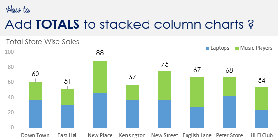
How to add totals to your stacked chart? - Goodly

Add Value Label to Pivot Chart Displayed as Percentage If you use the hidden line method: How to Add Total Data Labels to the Excel Stacked Bar Chart and then use the code mentioned in post #2 to create boxes offset from the hidden line points, you should be able to place the additional labels where you want. You must log in or register to reply here. Similar threads E

Excel Pivotchart not showing end of data labels - Super User

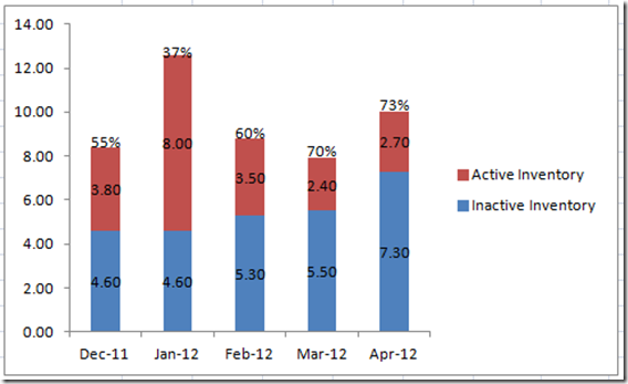
Include Grand Totals in Pivot Charts - My Online Training Hub Step 5: Format the Chart. The Grand Total value is the top segment of the stacked column chart. We need to hide this, but first let's select the grand total series and add Data Labels > Inside Base: Next, with the grand total series still selected go to the Format tab > Shape Fill > No Fill. Hide the gridlines and vertical axis, and place the ...

How to Sort Pivot Table Row Labels, Column Field Labels and Data Values with Excel VBA Macro ...

How to add data labels to pivot chart? | Console App Forums | Syncfusion The CSV data goes into the Data sheet and the application then creates a pivot table and corresponding pivot chart from this data in the Charts sheet. The chart is created alright but i see no option to add data labels to it using XlsIO. The chart is created as follows: IChartShape pivotChart = chartsSheet.Charts.Add();

Sort data in a PivotTable or PivotChart - Excel

Excel tutorial: Dynamic min and max data labels Now, back in the label options area, I'll uncheck Value, and check "Value from cells". Then I need to select the new column. When I click OK, the existing data labels are replaced by the labels I typed by hand. So that's the concept. Now we need to make the solution dynamic, and pull in the actual values. I'll start by adding the max value.

Pivot Table Row Labels In the Same Line - Beat Excel!

How to Add a Column to a Pivot Table - Excel Tutorials Add a Column to a Pivot Table. Now that we have our data into the Pivot Table, we will put players into the row field and averages of points into the value fields: If you, for whatever reason, wanted a different value (for example, a total sum of points) all you have to do is click the field in values (in this case Average of Points) and select ...

Create a pie chart from distinct values in one column by grouping data in Excel - Super User

Add a data label on Pivot Chart With .SeriesCollection (1).Points (i) .HasDataLabel = True .DataLabel.Text = Worksheets ("Sheet2").Range ("a" & position_total).Value position_total = position_total + 1 End With End With Next End Sub Select the Pivot chart, then run the macro "data_label". Jaynet Zhang TechNet Community Support

Pivot table row labels in separate columns • AuditExcel.co.za

Adding Data Labels to a Chart Using VBA Loops - Wise Owl To do this, add the following line to your code: 'make sure data labels are turned on. FilmDataSeries.HasDataLabels = True. This simple bit of code uses the variable we set earlier to turn on the data labels for the chart. Without this line, when we try to set the text of the first data label our code would fall over.

Creating Databound ADF Data Visualization Components

Formal ALL data labels in a pivot chart at once How do I format all data labels for all series in a chart at once? I frequently make pivot charts with multiple data series (line graphs). I know how to click on a data point and use the pane on the right to format the labels for that series, but it only changes that series.

Use Google Forms to make a Pivot Chart - TechnoKids News and Blog Posts

How to change/edit Pivot Chart's data source/axis/legends in Excel? Actually, it's very easy to change or edit Pivot Chart's axis and legends within the Filed List in Excel. And you can do as follows: Step 1: Select the Pivot Chart that you want to change its axis and legends, and then show Filed List pane with clicking the Filed List button on the Analyze tab.. Note: By default, the Field List pane will be opened when clicking the pivot chart.