45 excel pivot table conditional formatting row labels

Excel VBA: Conditional Format of Pivot Table based on ... For example, if you have the following table from which you create a pivot: Product Price Cola 123 Fanta 456 Sum of Price 789 then by creating a pivot table, you will have these items: Cola, Fanta, 'Sum of Price', and the following field labels: 'Row labels', 'Sum of Price'. How to Apply Conditional Formatting in Pivot Table? (with ... To apply conditional formatting in the pivot table, first, we must select the column to format. In this example, select "Grand Total Column." Then, in the "Home" Tab in the "Styles" section, click on "Conditional Formatting." Consequently, a dialog box pops up. Then, we need to click on "New Rule." As a result, another dialog box will pop up.

Excel tutorial: How to highlight rows with conditional ... To highlight rows in the table that contain tasks assigned to Bob, we need to take a different approach. First, select all of the data in the list. Then, choose New Rule from the conditional format menu on the Home tab of the ribbon. For style, choose "Classic". Then select "Use a formula to determine which cells to format".

Excel pivot table conditional formatting row labels

Apply Conditional Formatting | Excel Pivot Table Tutorial Go to Home Tab → Styles → Conditional Formatting → New Rule. From rule to, select the third option. And, from "select a rule" type select "Format only top or bottom" ranked values. In edit rule description, enter 1 in the input box and from the drop-down menu select "each Column Group". Apply formatting you want. Click OK. Excel Pivot Table Conditional Formatting Row Labels Go making the conditional formatting select the color scale and do it based on commercial and choose diverging and the colors should give expected result. Here a glaze color or bar and been applied... conditional formatting per row on pivot - Microsoft Tech ... conditional formatting per row on pivot. Hi, I would like to format each row of a pivot table separately (as in the picture shown below), but I cannot paste the formatting. I've got many rows, and they could change (just like the columns)

Excel pivot table conditional formatting row labels. Apply conditional formatting for each row in Excel Then click Format button, in the Format Cells dialog, under Fill tab, select green color. Click OK > OK. 4. Then drag the AutoFill handle to adjacent rows which you want to apply the conditional rule to, then in select Fill Formatting Only from the Auto Fill Options. Sample File Click to download the sample file Overwrite pivot table conditional format based on row label For your original question about how to overwrite pivot table conditional format based on a specific row label text, as Chitrahaas mentioned above, the formatting of the cell will be blank and if both conditions are true, so we're afraid that there is no out of box way to achieve your requirement directly. However, we found VBA code may ... Conditional Format Pivot Table Cell based on another cell ... Hi there I am working on a pivot table that highlights cells based on a Min. Value. However I would like the ability to color code the conditional formatting based on the product which is listed in the product column... apple, turnip, carrot etc. Make the apple cell red, carrot orange etc. On a side note I originally created custom number formatting to the Row column table. Design the layout and format of a PivotTable In the PivotTable Options dialog box, click the Layout & Format tab, and then under Layout, select or clear the Merge and center cells with labels check box. Note: You cannot use the Merge Cells check box under the Alignment tab in a PivotTable. Change the display of blank cells, blank lines, and errors

Conditional formatting rows in a pivot table based on one ... I am havong difficulty trying to highlight an entire row in a pivot table based on one rows criteria. The pivot table is from A:M and I need to highlight the corresponding row if column I has 992 in it. I have tried sevral ways but can only get it to work if I just focus on one row. I am at a loss for what I am doing wrong. Pivot Table Conditional Formatting with VBA - Peltier Tech It seems to occur because in 2007, conditional format is applied to a field, whereas in 2003, it's applied to a range. Without resorting to macros, it's possible to quickly reapply the conditional format in 2007 by following these steps: - Set the conditional format to range covering more than the pivot table (e.g. on cell above). Conditional Format Pivot Table Row | Chandoo.org Excel ... Excel Ninja Apr 3, 2013 #2 Select the entire row, and when you apply the conditional format, make the column reference absolute. So, say we want the entire row 2 to be formatted if cell in col B = 5. formula would be: =$B2=5 Conditional formatting for Pivot Tables in Excel 2016 ... The format I used was to select Conditional Formatting > Top 10 Items > set it to 1 item and select the default format. This format can be copied from one range to the next if desired or built up for each range individually. To copy the format, select one or more cells with that format and click Copy.

Conditional Formatting on Pivot Table row labels As per my knowledge, in this case it does not matter what is the source of pivot as after getting the data in pivot, it's the pivot where the conditional formatting need to be applied, please upload a sample. thanks. Regards, DILIPandey DILIPandey +91 9810929744 dilipandey@gmail.com Register To Reply Pivot Table Row Labels In the Same Line - Beat Excel! After creating a pivot table in Excel, you will see the row labels are listed in only one column. But, if you need to put the row labels on the same line to view the data more intuitively and clearly as following screenshots shown. Pivot table conditional format based on row value ... Hi there, I am hoping there is a way to use conditional formatting to change the fill color of the data cells on a pivot table based on the row value. In the picture below you can see I have grouped some values together to form the row categories - I would like to tell excel to fill the cells... Re-Apply Pivot Table Conditional Formatting - yoursumbuddy In cases where the conditional formatting might not apply to the leftmost row label, I've still applied it to that column, but modified the condition to check which column it's in. This function can be modified and called from a SheetPivotTableUpdate event, so when users or code updates a pivot table it re-applies automatically.

Sorting a Pivot Table - Free Microsoft Excel Tutorials

How to rename group or row labels in Excel PivotTable? To rename Row Labels, you need to go to the Active Field textbox. 1. Click at the PivotTable, then click Analyze tab and go to the Active Field textbox. 2. Now in the Active Field textbox, the active field name is displayed, you can change it in the textbox.

How to Create a MS Excel Pivot Table – An Introduction | SIMPLE TAX INDIA

Pivot Table with Conditional Formatting - Microsoft Community Ok, Pivot Tables are good, Pivot Tables are our friends. Now I want to use conditional formatting with a pivot table. I have seen a lot of examples, but none showing me how to use a field in the field list in the formula of a conditional format. Perhaps this is not possible, so I moved the field into a row label.

Design your Pivot Table in Excel | Excel in Excel

Format Pivot Table Labels Based on Date Range - Excel ... Select all the dates in the Row Labels that you want to format. On the Ribbon, click the Home tab, and then in the Styles group, click Conditional Formatting. In the list of conditional formatting options, click Highlight Cells Rules, and then click A Date Occurring.

How To Find And Remove Duplicates In A Pivot Table - MS Excel | Excel In Excel

Excel Conditional Formatting in Pivot Table - EDUCBA Click on any cell in the pivot table > Go to the HOME tab > Click on Conditional Formatting option under Styles option > Click on Manage Rules option. It will open a Rules Manager dialog box. Click on the Edit Rule tab, as shown in the below screenshot. It will open the Editing Rule formatting window. Refer to the below screenshot.

Re-Apply Pivot Table Conditional Formatting - yoursumbuddy

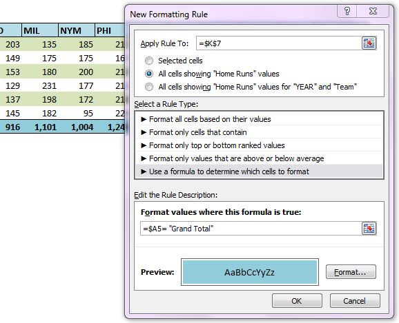
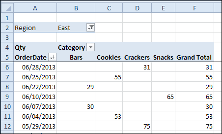
Pivot Table: Pivot table conditional formatting - Exceljet Select any cell in the data you wish to format and then choose "New rule" from the conditional formatting menu on the Home tab of the ribbon. At the top of the window, you will see setting for which cells to apply conditional formatting to. For the example shown, we want: "All cells showing sum of "sales values" for name and "date"

How to Apply Data Bars in Pivot Table - MS Excel | Excel In Excel

Pivot Table Conditional Formatting Weekend Data Highlight Add Conditional Formatting Follow these steps to apply the weekend highlighting in the pivot table: Select all cells where conditional formatting should be applied, cells B5 to B20 in this example. On the Excel Ribbon, click the Home tab Click Conditional Formatting, and in the drop down menu, click New Rule The New Formatting Rule dialog box opens

Format Pivot Table Labels Based on Date Range – Excel Pivot Tables

How to Apply Conditional Formatting to Rows ... - Excel Campus On the Home tab of the Ribbon, select the Conditional Formatting drop-down and click on Manage Rules…. That will bring up the Conditional Formatting Rules Manager window. Click on New Rule. This will open the New Formatting Rule window. Under Select a Rule Type, choose Use a formula to determine which cells to format.

Share :