39 excel chart legend labels

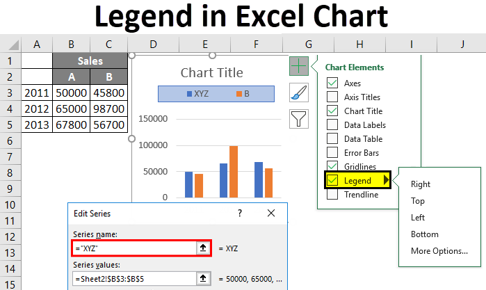
How to Add legends in Excel Chart? - WallStreetMojo Select the "Left" option from the "Legend,' and we may see the legends on the left side of the chart. Legends at the Top Right Side of the Chart Go to "More Options," select the "Top Right" option, and see the following result. If you are using Excel 2007 and 2010, the positioning of the legend will not be available, as shown in the above image. Excel Chart Legend | How to Add and Format Chart Legend? To bring the "Legend" on the chart, we must go to the Chart Tools - Design - Add chart element - Legend - Top. An extra element appears on the chart below as soon as we do this. That is called a "Legend." A legend gives us a direction as to what is marked in the chart in blue. In our example, it is the "Ratings" from customers.

How to Use Cell Values for Excel Chart Labels Select the chart, choose the "Chart Elements" option, click the "Data Labels" arrow, and then "More Options.". Uncheck the "Value" box and check the "Value From Cells" box. Select cells C2:C6 to use for the data label range and then click the "OK" button. The values from these cells are now used for the chart data labels.

Excel chart legend labels

Professional Quality Excel Chart Labels, Legends, and Colors The following Excel chart shows that Excel really CAN generate professional-quality chart figures. Here are some general strategies to consider…. 1. Set up your data-plumbing correctly. Here, the figure references a Staging Table, which references a Data Table maintained by Power Query, which updates the data from the Web in less than five ... Add a legend to a chart - support.microsoft.com Click the chart. Click Chart Filters next to the chart, and click Select Data. Select an entry in the Legend Entries (Series) list, and click Edit. In the Series Name field, type a new legend entry. Tip: You can also select a cell from which the text is retrieved. Click the Identify Cell icon , and select a cell. Click OK. Excel Chart not showing SOME X-axis labels - Super User Apr 05, 2017 · What worked for me was to right click on the chart, go to the "Select Data" option. In the box, check each Legend Entry and ensure the corresponding Horizontal Labels are fully filled in. I found for me only one Legend had the full X-axis list, but there was one that didn't and this meant half of my X-axis labels were blank.

Excel chart legend labels. Insert a chart from an Excel spreadsheet into Word Keeps the Excel theme. Keeps the chart linked to the original workbook. To update the chart automatically, change the data in the original workbook. You also can select Chart Tools> Design > Refresh Data. Picture. Becomes a picture. You can’t update the data or edit the chart, but you can adjust the chart’s appearance. Under Picture Tools ... How to remove a legend label without removing the data series In previous versions of Excel, I have been able to simply click on and delete any unwanted legend labels, whilst leaving the data series and chart unchanged. In Excel 2016, it appears that individual legend labels cannot be removed from the legend without also removing their associated data series. I simply want to remove individual legend ... How To Add and Remove Legends In Excel Chart? - EDUCBA Click on the "+" symbol on the top right-hand side of the chart. It will give a popup menu with multiple options as below. By default, Legend will be select with a tick mark. If we want to remove the Legend, remove the tick mark for Legend. We removed the tick mark; hence the Legend is removed from the chart we can observe in the below picture. Comparison Chart in Excel | Adding Multiple Series Under Same … This window helps you modify the chart as it allows you to add the series (Y-Values) as well as Category labels (X-Axis) to configure the chart as per your need. Under Legend Entries ( S eries) inside the Select Data Source window, you need to select the sales values for the year 2018 and year 2019.

Use a screen reader to add a title, data labels, and a legend to a ... Select the chart that you want to work with. To open the Add Chart Element menu, press Alt+J, C, A. To add data callout labels to the chart, press D and then U. Tip: To remove data labels, select the chart, and then press Alt+J, C, A, D, and then N. Add a legend to a chart Legends help you to quickly understand data relationships in a chart. How to Add Labels to Scatterplot Points in Excel - Statology Step 3: Add Labels to Points. Next, click anywhere on the chart until a green plus (+) sign appears in the top right corner. Then click Data Labels, then click More Options…. In the Format Data Labels window that appears on the right of the screen, uncheck the box next to Y Value and check the box next to Value From Cells. Excel Chart Vertical Axis Text Labels • My Online Training Hub Apr 14, 2015 · So all we need to do is get that bar chart into our line chart, align the labels to the line chart and then hide the bars. We’ll do this with a dummy series: Copy cells G4:H10 (note row 5 is intentionally blank) > CTRL+C to copy the cells > select the chart > CTRL+V to paste the dummy data into the chart. Excel Chart not showing SOME X-axis labels - Super User 05/04/2017 · In Excel 2013, select the bar graph or line chart whose axis you're trying to fix. Right click on the chart, select "Format Chart Area..." from the pop up menu. A sidebar will appear on the right side of the screen. On the sidebar, click on "CHART OPTIONS" and select "Horizontal (Category) Axis" from the drop down menu.

Excel Column Chart with Primary and Secondary Axes - Peltier Tech 28/10/2013 · The second chart shows the plotted data for the X axis (column B) and data for the the two secondary series (blank and secondary, in columns E & F). I’ve added data labels above the bars with the series names, so you can see where the zero-height Blank bars are. The blanks in the first chart align with the bars in the second, and vice versa. Show or hide a chart legend or data table If you have space constraints, you may be able to reduce the size of the chart by clearing the Show the legend without overlapping the chart check box. Show or hide a data table Click the chart of a line chart, area chart, column chart, or bar chart in which you want to show or hide a data table. How to Create a Milestone Chart in Excel Steps to Create a Milestone Chart in Excel. I have split the entire process into three steps to make it easy for you to understand. 1. Set Up Data ... our chart is totally blank. So, we have to re-assign series and axis labels. Click on “Add” from legend entries. In edit series window, enter “Date” in the series name and select activity ... Add or remove data labels in a chart - support.microsoft.com Click the data series or chart. To label one data point, after clicking the series, click that data point. In the upper right corner, next to the chart, click Add Chart Element > Data Labels. To change the location, click the arrow, and choose an option. If you want to show your data label inside a text bubble shape, click Data Callout.

30 How To Label Legend In Excel - Label Design Ideas 2020

Excel: How to Create a Bubble Chart with Labels - Statology Step 3: Add Labels. To add labels to the bubble chart, click anywhere on the chart and then click the green plus "+" sign in the top right corner. Then click the arrow next to Data Labels and then click More Options in the dropdown menu: In the panel that appears on the right side of the screen, check the box next to Value From Cells within ...

How to Make a Chart or Graph in Excel [With Video Tutorial]

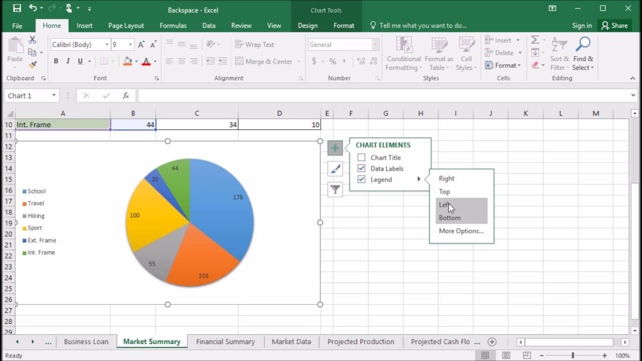
Excel Charts - Chart Elements - Tutorials Point Now, let us add data Labels to the Pie chart. Step 1 − Click on the Chart. Step 2 − Click the Chart Elements icon. Step 3 − Select Data Labels from the chart elements list. The data labels appear in each of the pie slices. From the data labels on the chart, we can easily read that Mystery contributed to 32% and Classics contributed to 27% ...

408 How format the pie chart legend in Excel 2016 - YouTube

Arranging Trendline Labels in Excel Chart Legend - It won't follow ... Arranging Trendline Labels in Excel Chart Legend - It won't follow the Select Data order I've got a chart in Excel on Windows that will not change the order of the entries in the legend. I've got scatterplots with trendlines and they're labeled "2017" on up to "2021" but for some reason 2019 will not go in the right order.

Excel Chart Elements: Parts of Charts in Excel | ExcelDemy

Directly Labeling in Excel - Evergreen Data There are two ways to do this. Way #1 Click on one line and you'll see how every data point shows up. If we add a label to every data points, our readers are going to mount a recall election. So carefully click again on just the last point on the right. Now right-click on that last point and select Add Data Label. THIS IS WHEN YOU BE CAREFUL.

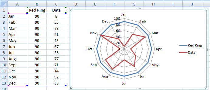
Excel Dashboard Templates How-to Highlight or Color Rings in an Excel Radar Chart - Excel ...

Chart.Legend property (Excel) | Microsoft Docs Returns a Legend object that represents the legend for the chart. Read-only. Syntax. expression.Legend. expression A variable that represents a Chart object. Example. This example turns on the legend for Chart1 and then sets the legend font color to blue. Charts("Chart1").HasLegend = True Charts("Chart1").Legend.Font.ColorIndex = 5 Support and ...

Excel Chart Data Series, Data Points, Data Labels

Change legend names - support.microsoft.com Select your chart in Excel, and click Design > Select Data. Click on the legend name you want to change in the Select Data Source dialog box, and click Edit. Note: You can update Legend Entries and Axis Label names from this view, and multiple Edit options might be available. Type a legend name into the Series name text box, and click OK.

Position Chart Legend & Display Gridlines in Microsoft Excel: MOOC - YouTube

How to Edit Legend in Excel - Excelchat Add legend to an Excel chart Step 1. Click anywhere on the chart Step 2. Click the Layout tab, then Legend Step 3. From the Legend drop-down menu, select the position we prefer for the legend Example: Select Show Legend at Right Figure 2. Adding a legend The legend will then appear in the right side of the graph. Figure 3.

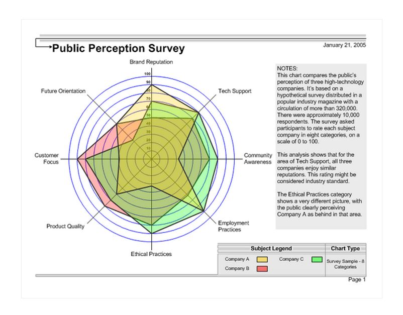
Spider Chart | Spider Chart Template | Free Spider Chart

How to Add Total Data Labels to the Excel Stacked Bar Chart Apr 03, 2013 · For stacked bar charts, Excel 2010 allows you to add data labels only to the individual components of the stacked bar chart. The basic chart function does not allow you to add a total data label that accounts for the sum of the individual components. Fortunately, creating these labels manually is a fairly simply process.

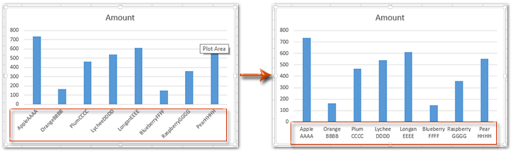
How to wrap X axis labels in a chart in Excel?

Chart axes, legend, data labels, trendline in Excel - Tech Funda To position the Data Labels in excel, select 'DESIGN > Add Chart Element > Data Labels > [appropriate command]'. For example, in below example, the data label has been positioned to Outside End. To format the Data Labels, select 'More Data Label Options...' and select approproate formatting from right side panel. Bringing Data Table on the chart

5 Easy Steps to Make Your Excel Charts Look Professional | Easy-Excel.com

Excel charts: how to move data labels to legend - Microsoft Tech Community You can't do that, but you can show a data table below the chart instead of data labels: Click anywhere on the chart. On the Design tab of the ribbon (under Chart Tools), in the Chart Layouts group, click Add Chart Element > Data Table > With Legend Keys (or No Legend Keys if you prefer)

30 How To Label Legend In Excel - Label Design Ideas 2020

9 Ways to Edit Legends in Excel - Ultimate Guide - QuickExcel Editing Legends in Select Data Right-click on the chart. Click on Select Data. Look on the left side under Legend Entries. Select the legend name you want to change. Click on Edit. Enter a new name for that legend under Series Name. New Name Added Another way you can edit the legend names can be as follows. Click on the chart. Go to the Design tab.

Excel Charts: Dynamic Label positioning of line series

How do I change a chart legend's icon and font sizes in Excel ... Replied on July 23, 2013. You must click once on the legend box to select it. Don't double-click it. Then you right click your mouse while the legend is still selected. It will open a little dialogue box where it will allow you to change the font type & font size etc. Report abuse.

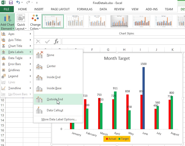
Chart axes, legend, data labels, trendline in Excel - Tech Funda

How to change the order of your chart legend - Excel Tips & Tricks ... Under the Data section, click Select Data. Step 2: In the Select Data Source pop up, under the Legend Entries section, select the item to be reallocated and, using the up or down arrow on the top right, reposition the items in the desired order.

A Beginner's Guide on How to Plot Graph in Excel | Alpha Academy

Excel 2007 : Display legend entries in chart bars (similar to data labels) Display legend entries in chart bars (similar to data labels) I have a column chart where I would like to display the legend entries inside the columns, a bit like data labels are possible to display inside the pie pieces in a pie chart. In this way the viewer doesn't need to look in a legend and compare colours to figure out which bar is which.

Dynamically Label Excel Chart Series Lines • My Online Training Hub

Line charts: Moving the legends next to the line - Microsoft Tech Community With data labels you may simplify the procedure. Click on line, it shows you data points, when click on one point (other ones wan't be shown) and from right click Add data label Into the box which appears you may put any text and format it as you want If you have data labels initially just format the data label for one of points on your choice.

How To Label Legend In Excel Pie Chart - Chart Walls

Excel charts: add title, customize chart axis, legend and data labels Click the Chart Elements button, and select the Data Labels option. For example, this is how we can add labels to one of the data series in our Excel chart: For specific chart types, such as pie chart, you can also choose the labels location. For this, click the arrow next to Data Labels, and choose the option you want.

Excel charts: add title, customize chart axis, legend and data labels

How do I make chart labels or legends wordwrap? [SOLVED] > cell containing the legend entry text, using Alt+Enter). > > You have no control over axis tick labels, other than hard-coding a carriage > return in the cell containing the tick label text, using Alt+Enter. > Sometimes these wrap where Excel wants them to, but you can't control the > label size. >

Share :